
The classification problem for this project was inspired by a silly hypothetical question I thought of: could you make an entire NFL team out of Cam Newton clones? Cam Newton is a exceptional athlete, running a 4.56 second 40-yard dash at 6’ 5” and 250 lbs. While he currently plays quaterback, it stands to reason that with his strength and size he could excel at other positions on the field (related article). This got me thinking about the average statistics of each position and how Cam compares. This then led me to think about whether player position could be reasonably classified based on some basic player statistics.
Tools
For this project I used the scikit-learn library for Python for the machine learning algorithms and matplotlib for visualization.
Dataset
The data I used for my analysis comes from a dataset available on Kaggle called NFL Combine. The NFL Scouting Combine is an event where prospective NFL players demonstrate attributes like strength and speed to teams. The dataset has 5636 samples and covers the years from 2000 to 2017. It includes player attributes like height, weight, performance on exercises, and position.
The first preprocessing step I needed to do was convert height from a ft-in string to inches as an integer type. I also needed to address records with missing data. Not every player does every test at the Combine so many fields were empty (~19%). Many of the algorithms I used can not handle missing data, so I decided to impute the missing values with the mean of the column.
To start off, I wanted to visualize relationships between some features. The plots below pair the Height, Weight, and 40-yard dash times (Cam Newton’s stats are indicated with a blue triangle).
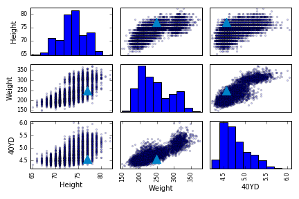
Some fairly intuitive trends can be seen like weight increasing as height increases and 40-yard dash time increasing as weight increases. In both the 40YD vs Weight and 40YD vs Height plots it can be seen that Cam is relatively fast given his size. The histogram for weight shows that there is a main peak at around 210 lbs with a second smaller peak around 320 lbs. This second peak may correspond to a specific player position.
Algorithms
Decision Tree
The first algorithm I used to classify player position was a decision tree. The sklearn decision tree algorithm requires numeric features. Because of this I had to convert categorical values into binary columns.
I utilized the grid-search functionality in sklearn to find the hyperparameter settings that returned the best results on the training set. The hyperparameters I tuned for the DT were minimum samples leaf and split criterion. The mean training and test scores from 3 fold cross validation for the different parameter values are shown below:
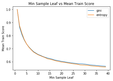

The difference between either gini or entropy as the split criterion was fairly negligible. The training score decreases as the minimum sample leaf size increases which makes sense. When the minimum leaf size is set to 1, it will allow to algorithm to successfully classify each training record. Conversely, the opposite is true for the test score as it increases with minimum sample leaf size up to a point. This shows overfitting is reduced, and the algorithm can generalize better. The best result (52.9%) was observed with the entropy criterion and with minimum sample leaf size set to 21.
Support Vector Machine
The next algorithm I used was the Support Vector Machine implementation in sklearn. Part of the reason I decided to use SVM is because it is the suggested algorithm for my dataset characteristics based on this useful flow diagram. Specifically it recommends using a linear kernel. I also experimented with the radial basis function (rbf) kernel. The plots below show penalty parameter values vs training/testing cross validation scores for both the linear and rbf kernel.


I found the highest mean test cross validation score (56.5%) occurred with the linear kernel and the penalty parameter set to 10. When the penalty parameter is very low the margin of the hyperplane is increased which increases the amount of misclassified training data. The training accuracy for the rbf kernel increases remarkably as the penalty parameter increases from 0.1 to 1. Both the training and testing CV scores begin to plateau for the linear kernel as the penalty parameter increases.
Random Forest
The last algorithm I evaluated was a random forest classifier. It is an ensemble learning that combines the output of multiple decision trees. The number of decision trees to use is an important parameter to consider. Like with the decision tree, the available split criteria are gini and entropy. The output of the grid search is shown below:

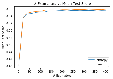
Classification accuracy improved sharply as the number of estimators used increased until around 100 after which it levels off. Again like with the decision tree, the choice of criterion did not have a large impact but the gini split criteria does appear to perform better on average. The best result (55.8%) was observed with 320 estimators and gini split criterion. Using these settings, I also experimented with the maximum number of features to consider when determining a split. The plot below uses the average of 10 runs:

The best result 56.1% with a maximum of 3 features.
Results
The SVM classifier performed the best on the training set with a cross validation test accuracy of 56.5%. The performance on the test set with the same parameters was 57.2%. The fact that the test accuracy was slightly higher than the CV accuracy indicates that the algorithm did a good job not overfitting on the training data.
The confusion matrix below (generated with seaborn library) shows the actual player position in the rows and predicted positions in the columns for the test set.

The algorithm performed best classifying quarterbacks and running backs with 74% and 73% accuracy respectively. It’s possible both positions have unique characteristics that made them easier to classify. In general, QBs are relatively unathletic compared to other players the same size while RBs tend to be shorter. Further analysis would need to done to know for sure.
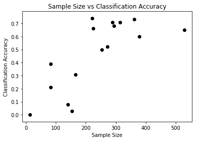
The classification accuracy of player position is correlated with the number of samples in the dataset as shown in the graph below. This may be due to many positions having similar attributes. In this scenario the algorithm would reduce errors by classifying a test sample as the better represented position. For example players in the Free Safety position were primarily predicted to be either Cornerbacks (25%) or Wide Receivers (56%), both of which have 3 to 4 times the samples in the dataset. Free Safeties tend to be relatively slim and fast much like CBs and WRs.
The pie chart below shows the class probabilities for Cam Newton. Sklearn uses Platt scaling to determine the probability estimates.

From the results, Cam clearly does not fit the mold of a standard quarterback. QB was the fifth highest probability with Tight End being the position returned as the predicted class. Three defensive positions had a higher probability than QB indicating Cam’s potential versatility. The attributes in the Combine dataset do not capture the full skill set required to excel at a position, but based on these statistics alone it appears that Cam could play multiple positions.
Possible Enhancements
The data I have used is from the Combine which contains information for all prospects, including those who never play in the NFL. It would be interesting to add data around NFL career statistics to see how well the various attributes in the Combine dataset predict future success in the NFL. This type of analysis has doubtlessly been performed by actual NFL teams and represents a real world problem.
It would also be interesting to see how this algorithm performs against football experts like coaches and scouts. It would require trials where the experts are asked to classify player position based on the combine stats alone. My intuition is they would perform well but the algorithm may have an edge.
Feature evaluation could be performed to discover which features had the biggest impact on classifying player position. A procedure like Principal Component Analysis would be useful to determine which features contain the most information about the dataset.
Unfortunately I do not believe the initial question of this exercise can be answered until cloning technology advances further.
References
http://scikit-learn.org/stable/modules/grid_search.html#grid-search
http://scikit-learn.org/stable/tutorial/machine_learning_map/index.html
https://scikit-learn.org/stable/modules/generated/sklearn.svm.SVC.html